Launch Watch · Evidence study
Published
Huntington Beach oil-spill images: the 16-hour comparison gap
Two real 2021 spill images reveal different observables. Reproduce their 16-hour-33-minute time gap before comparing Landsat and Sentinel-1B.
Two satellite views of the 2021 Huntington Beach oil spill look dramatically different. One is a hazy natural-color coastline; the other has conspicuous dark features on the water. It is tempting to treat them as a simple test of which sensor is better at seeing oil.
The timestamps complicate that story. The two acquisitions were 16 hours and 33 minutes apart, and the instruments observed different physical properties. A careful comparison can explain the contrasting appearance, but it cannot isolate a same-time sensor-performance advantage.
The worked check below uses the two NASA-produced images and the acquisition times in NASA Earth Observatory’s account. Its original contribution is an exact time difference plus a sensor-and-time audit, rather than a new spill outline.
Put both observations on the same clock
| Image | Time reported in California | UTC acquisition | Observable |
|---|---|---|---|
| Sentinel-1B | October 2, 2021, 6:49 p.m. PDT | 2021-10-03T01:49:00Z | Radar backscatter related to surface roughness |
| Landsat 8 | October 3, 2021, 11:22 a.m. PDT | 2021-10-03T18:22:00Z | Natural-color reflected-light appearance |
The radar acquisition happened first. In California it was the evening of October 2; in UTC it was already October 3. Landsat’s acquisition followed late the next morning in California. A date-only label can hide this separation because both are October 3 in UTC.
Using the published UTC times, the interval is 18:22 minus 01:49: 16 hours and 33 minutes, or 59,580 seconds. This arithmetic uses the source’s minute-level timestamps. It does not estimate how long the oil had been present or how much it moved during that interval.
That distinction helps when assembling an image comparison. The acquisition date belongs in the caption, but the acquisition time and timezone determine whether two views can reasonably be called simultaneous. Here they plainly cannot.
What the optical image actually shows
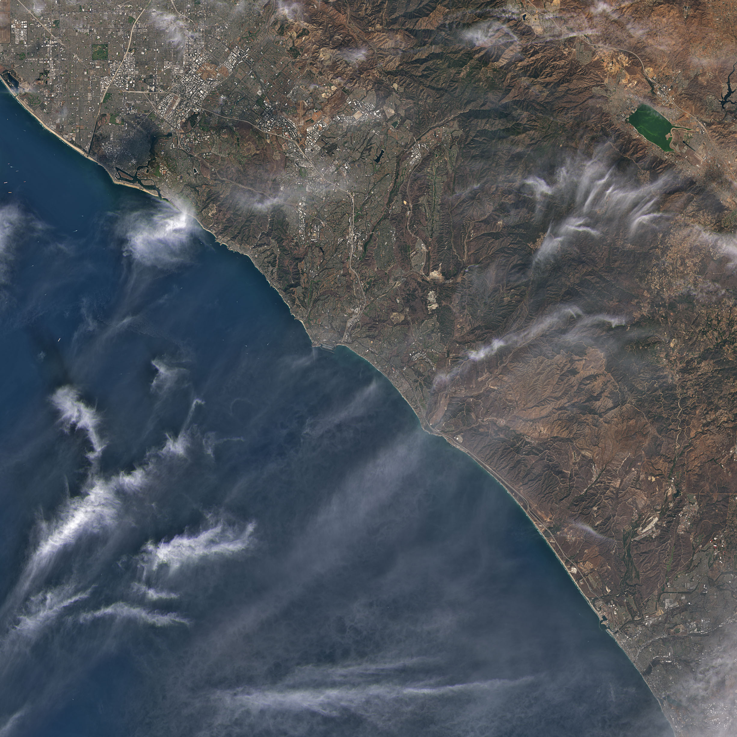
The Landsat 8 image is a natural-color rendering from its Operational Land Imager. The displayed scene has wispy clouds, haze and low-contrast ocean features. NASA describes faint hints of oil amid other visible features in this image.
An optical image offers familiar coastline and land context, but familiarity can make its meaning feel more direct than it is. A dark or light streak in a rendered scene is an appearance that needs interpretation. The image does not come with a chemically identified oil label at every pixel, and this reading does not turn its colors into oil thickness or volume.
The useful observation is specific: the water in this particular image does not present the same strong dark contrast seen in the radar view. That is a statement about two selected renderings, not a general optical detection limit.
What changes in the radar view
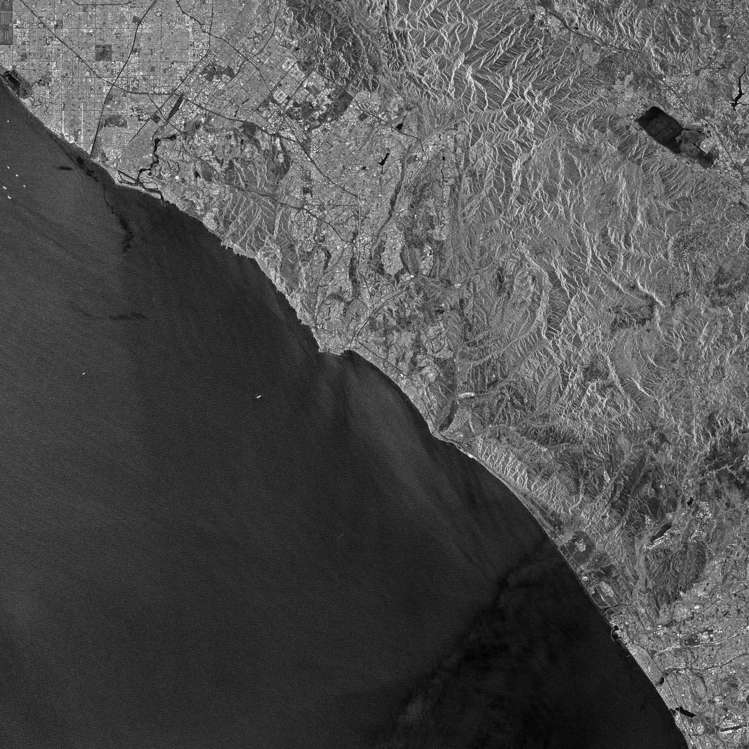
Sentinel-1B used synthetic aperture radar. In NASA’s explanation of this scene, rougher surfaces appear brighter and smoother surfaces darker. Oil can damp the small capillary waves on the sea surface, making an affected area smoother and altering its radar return.
In the selected radar rendering, elongated dark water features stand out against surrounding water and bright land. That appearance helps explain why radar is useful in the provider’s account of this spill. It does not make darkness a unique chemical signature. A low-backscatter patch requires interpretation; assigning every dark patch to oil would go beyond what the displayed quantity establishes by itself.
The visible contrast therefore has two pieces: the instrument responds to surface roughness, and the source interprets features in a documented spill setting. Keeping those pieces separate avoids presenting the radar display as a direct oil-composition map.
Separate contrast from a controlled comparison
| Comparison question | What changed | Conclusion supported |
|---|---|---|
| Why does the radar view have stronger dark features? | The physical observable and display both differ | The images demonstrate different kinds of surface contrast |
| Did one sensor detect more oil than the other? | Sensor type and acquisition time both change | The pair does not isolate sensor performance |
| How far did the slick move? | Time passes, but comparable feature identity is unestablished | No drift vector or speed is measured from these JPEGs |
A controlled comparison would need the question and reference conditions defined more tightly. If the aim were relative detection performance, a reviewer would ask how observation times, footprints, environmental conditions, processing and independent reference information were matched. These two presentation images do not settle those questions.
This does not make the pair unhelpful. Its strength is explanatory: it shows why reflected-light appearance and radar response can highlight different aspects of a coastal scene. Its weakness as a benchmark is equally clear: sensor type and observation time change together.
Check the claim: “The radar proves how far the oil moved before Landsat.”
The 16-hour-33-minute interval is established. A movement estimate is not. A comparable feature would first need to be identified in both observations with suitable geospatial and physical support. This article does not track one or compute a drift speed.
Show the timezone check
Sentinel-1B: October 2 at 18:49 PDT plus seven hours is October 3 at 01:49 UTC. Landsat 8: October 3 at 11:22 PDT plus seven hours is October 3 at 18:22 UTC. Subtracting gives 16 hours and 33 minutes. The timezone conversion changes the date of the first acquisition, not the elapsed time.
A caption that earns the comparison
A useful caption for this pair should name both instruments, identify reflected-light appearance versus radar backscatter, and state the time gap. Those details let the reader appreciate the contrast without quietly treating the pair as a simultaneous experiment.
This bounded reading uses the NASA-produced optical and radar derivatives. It does not use the inaccessible surveillance-report image, recover calibrated reflectance or backscatter, trace ship identities, assign fault, or estimate spill volume, thickness, area or severity. No new physical retrieval is claimed.
The transferable habit is simple: compare the observables and the clocks before comparing how persuasive the pictures look. Here, 16 hours and 33 minutes is the most important number the image pair itself does not make obvious.
Sources and image use
- NASA Earth Observatory: Satellites View California Oil Spill, October 8, 2021. Source for the selected image derivatives, acquisition times, sensor description and credits.
- NASA images and media guidelines, for factual editorial reproduction with attribution.
- Copernicus Sentinel legal notice. The radar derivative retains the required modified-data notice in its caption. Neither image implies agency endorsement.